Reading shape and motion out of V-JEPA
The question I wanted to answer was simple: what does V-JEPA actually represent inside its latent space? This is less straightforward than one might think.
I’ve been catching up on AI research since leaving my last role, and world models continue to fascinate me. While I have no doubts about the economic value of the current trajectory of LLMs, I don’t have a strong sense that it will translate cleanly into embodied AI. With some free time, I’ve been running whatever experiments I can locally to improve my understanding of the current state of the research.
LLMs are fairly straightforward, albeit in a completely unintuitive way. You take text, encode it in a higher-dimensional space, and adjust a huge number of parameters to squeeze as much semantic structure as possible out of the pretraining corpus. Somehow, through the wizardry of attention blocks, backpropagation, and ungodly amounts of compute, those parameters converge on useful semantics which you can decode into a probable token out the back.
JEPA (Joint-Embedding Predictive Architecture) tries to build a predictor that captures concepts about the world rather than directly reproducing its input. V-JEPA applies that idea to video. But what does it actually represent inside its latent space?
The setup
V-JEPA is Meta’s video model. You feed it frames, and it gives you back a stack of latent vectors. This is roughly what an LLM does to a sentence, except now the representation spans space and time. The values are continuous features rather than named classes. So how do I know what they contain?
At first I tried the most direct approach: feed the model a handful of real videos that looked roughly similar or different.
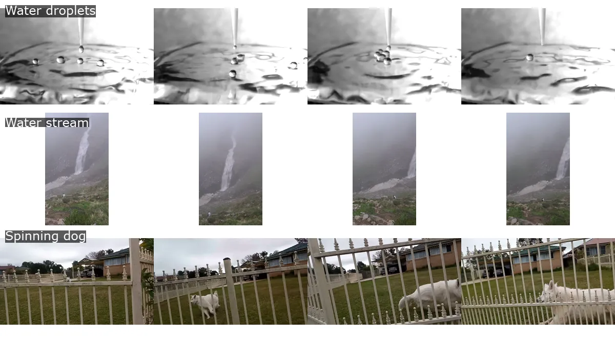
The first three videos were water droplets, a stream of water, and a spinning dog. I expected the distance between these embeddings to be different when sampled across different time periods. I didn’t really think through this too much but I was nevertheless surprised that two vertical water features were so dissimilar.
The cross-entropy values below are completely meaningless.
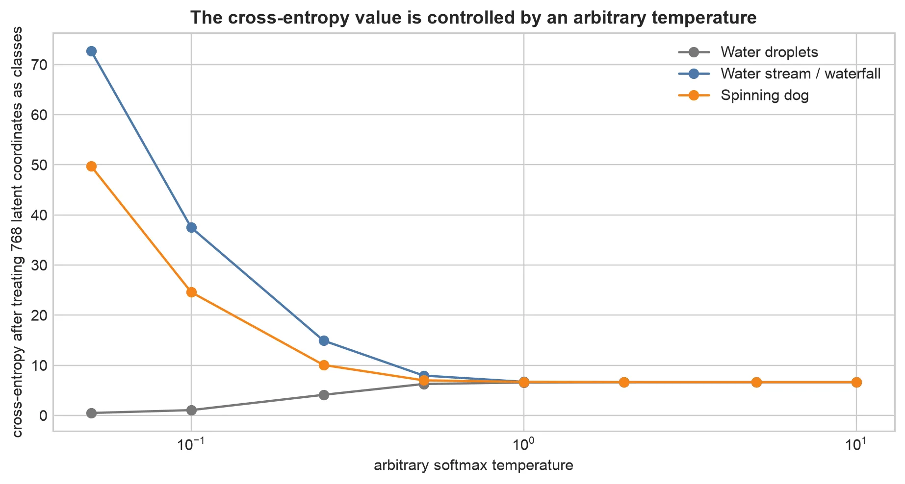
I had treated V-JEPA’s continuous latent features as if they were classes. They aren’t. Softmax and cross-entropy didn’t make sense here.
Next, I pooled each video’s tokens into one vector and calculated pairwise cosine distance.
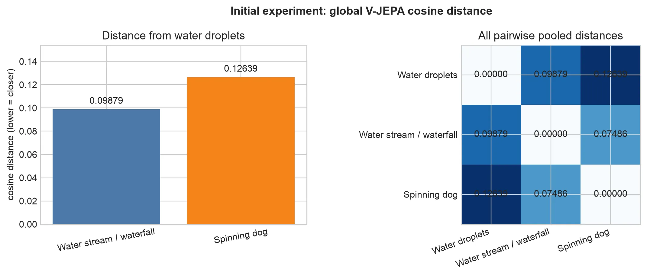
| Pair | Cosine distance |
|---|---|
| Droplets ↔ water stream | 0.099 |
| Droplets ↔ spinning dog | 0.126 |
| Water stream ↔ spinning dog | 0.075 |
The water stream sits closer to a spinning dog than to the other water clip. Pooling this aggressively was only a rough baseline, but the result made the limitation obvious.
I don’t think I picked bad videos for this experiment. Videos vary along many axes at once:
- Subject matter
- Background and setting
- Colour and texture
- Lighting
- Camera position and camera movement
- Composition
- Object appearance
- Type and amount of motion
- Time
There were two problems. I had pooled thousands of spatial-temporal tokens into one vector, then reduced the difference between two of those vectors to one number. It wasn’t clear what that number meant. So I tried a more controlled experiment: could I pull shape and motion out of the frozen representation?
I trained a linear probe to find out. A probe is just one matrix: no hidden layer and no nonlinearity. If something this simple can recover the label from frozen activations, then the information is already somewhere in those activations. V-JEPA never changes during this process.
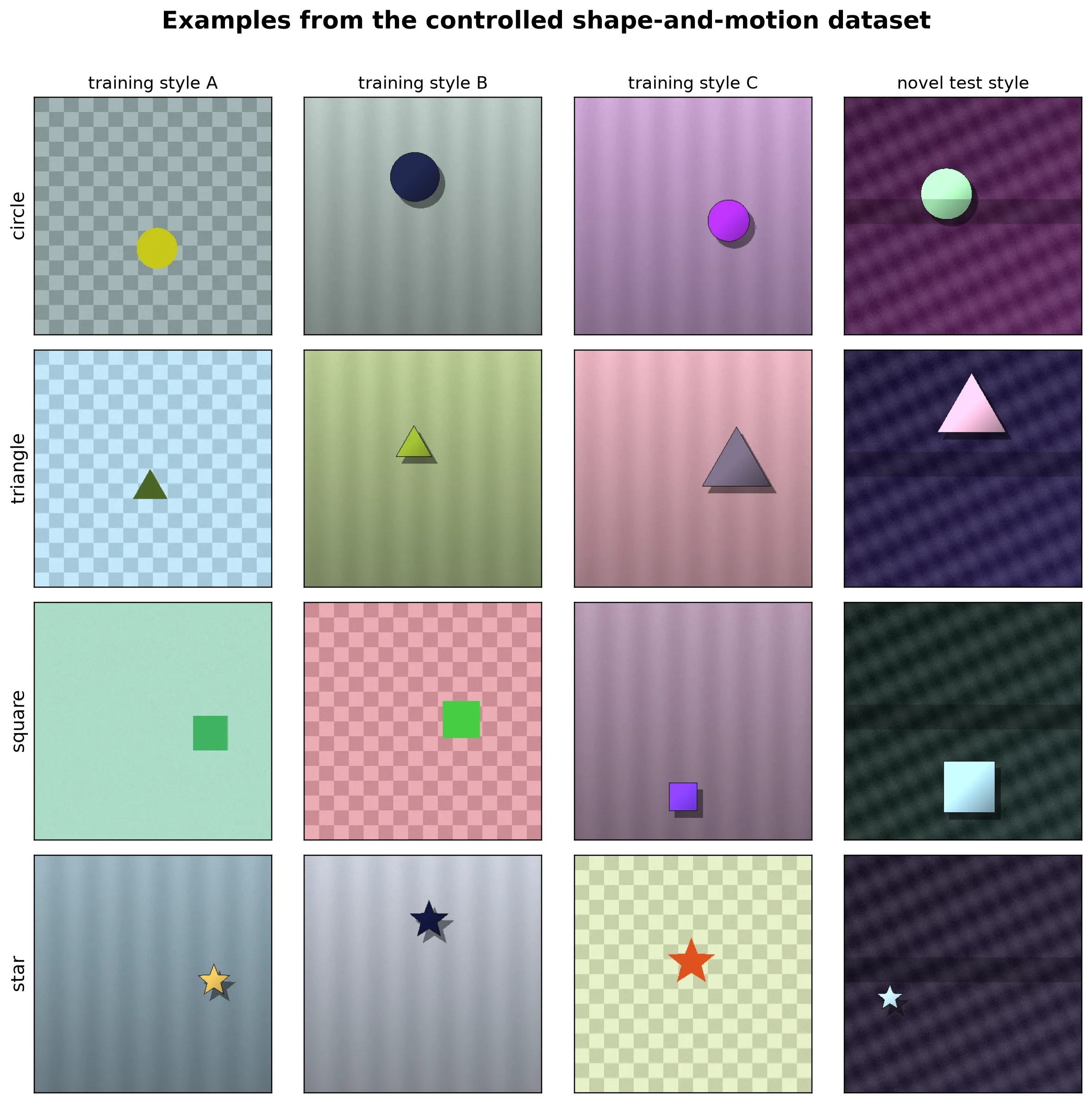
My videos were synthetic and simple: four shapes—circle, triangle, square, and star—and four directions—right, left, down, and up. I randomized factors that might leak the answer: size, starting position, colour, background, texture, lighting, and rendering style. Every shape appeared moving in every direction, so the probe could not infer “moving left” from “triangle.”
The short version:
| Test | Result |
|---|---|
| Four-way shape, novel renderer | 127/128 |
| Four-way direction, untouched test set | 126/128 |
| Direction on excluded object identities | 125/128 |
| Motion-separation AUC after the probe | 0.993 |
How V-JEPA represents each video
I fed V-JEPA 16 frames at 384 × 384. Two things happen. The patch embedding pairs adjacent frames. Frames 1–2 become temporal slice 1, 3–4 slice 2, and so on down to 15–16, so 16 frames become 8 temporal slices, each covering roughly two frames’ worth of a moment.
In space, the ViT-B/16 encoder chops each frame into 16-pixel patches: 384 / 16 = 24 across and 24 down, a 24 × 24 grid = 576 patches per frame.
This is part of V-JEPA’s architecture. Each spatiotemporal patch is called a tubelet.
2 frames × 16 × 16 px → V-JEPA → one 768-d tokenSo the full output is:
8 temporal × 24 × 24 spatial × 768 features = 8 × 24 × 24 = 4,608 tokensWhat happens next depends on the property being decoded. For motion, I averaged the 576 spatial tokens within each temporal slice, producing one 768-dimensional summary for each of the eight moments:
early₁, early₂, … late₇, late₈I averaged over space so I never told the probe where the object was. I did not average over time. Left-to-right and right-to-left clips visit the same places in opposite order, so combining the eight slices would throw away exactly what I was looking for. The shape probe used a different summary, which I’ll get to below.
Shape decoding
1. Generate synthetic videos
I programmatically generated synthetic videos containing:
- Circle
- Triangle
- Square
- Star
Each video had a known label. I then randomized motion, colour, position, size, background, texture, lighting, and rendering style.
2. Process the video
16 frames
↓
V-JEPA
↓
8 × 24 × 24 × 768 activations
I did not tell the decoder where the shape was.
To turn the many tokens into a fixed-size shape description, I calculated three statistics for each of the 768 feature dimensions across all spatial and temporal tokens:
- Mean
- Standard deviation
- Maximum
mean activation: 768 numbers
activation variation: 768 numbers
maximum activation: 768 numbers

concatenated:
2,304 numbers
Why use these three?
- Mean captures features broadly present throughout the video.
- Standard deviation captures how unevenly or variably features activate.
- Maximum preserves strong local responses that averaging might dilute.
3. Train linear layer
I trained one linear layer to classify those 2,304 values as [circle, triangle, square, star].
During training:
- The probe produced four scores for each video.
- Softmax converted those meaningful class scores into probabilities.
- Cross-entropy compared them with the known shape label.
- Only the linear probe’s weights were updated.
This is where softmax and cross-entropy were appropriate: the four output coordinates had explicit meanings corresponding to mutually exclusive shape classes.
Shape evaluation
I tested the probe on 128 independently generated videos using a novel visual style:
- Darker backgrounds
- Different textures
- Outlined shapes
- Different lighting and shadows
- Partial occlusion
It correctly classified 127 of 128 videos. That is almost suspiciously good. I would not take this as proof that V-JEPA generally understands shapes: these were clean, isolated, very different shapes, and every example came from a related programmatic renderer. I mostly needed the shape test to help separate motion from object identity.
Motion decoding
1. Generate synthetic videos
I generated videos with four motion labels:
- Right
- Left
- Down
- Up
Shape and direction were independent:
circle moving right
triangle moving right
square moving right
star moving right
I also randomized colour, size, position, speed, background, lighting, and texture.
This was meant to stop the probe from predicting direction using some unrelated shortcut.
2. Try the full temporal sequence
My first motion decoder concatenated all eight summaries (8 × 768 = 6,144 values):
[z₁, z₂, ..., z₈]
↓
6,144-value vector
↓
linear direction probe
This worked well on familiar-looking videos, but failed under a large change in rendering style.
The sequence still contained considerable static appearance information, allowing the probe to depend on the visual domain.
3. Test more motion-focused summaries
I tested three alternatives:
- Last slice minus first slice:
z₈ − z₁ - Subtract the video’s average activation from every slice.
- Calculate the difference between every adjacent pair:
z₂ − z₁, z₃ − z₂, …, z₈ − z₇
On the diagnostic novel-style set:
| Summary | Direction accuracy |
|---|---|
| Last minus first | 96.1% |
| Temporally centered sequence | 94.5% |
| Adjacent differences | 60.9% |
I selected last-minus-first. My hypothesis is that it would be less useful in a complex scene with multiple objects or several simultaneous motions; temporal centering might prove more robust there, but this experiment did not test that.
4. Construct the final motion feature
The final feature was ending activation − starting activation, or Δz = z₈ − z₁.
This produced one 768-dimensional change vector.
The idea was that static information would partially cancel:
background − background ≈ 0
object color − object color ≈ 0
while the change in state would remain:
object at ending position − object at starting positionThis is a rough activation-space equivalent of displacement.
5. Train the linear motion decoder
I trained one linear layer:
768-value change vector
↓
linear layer
↓
[right, left, down, up]
Its weight matrix had shape 4 × 768.
The four output coordinates were meaningful class logits, so I could appropriately use softmax and cross-entropy during probe training.
Only the linear layer changed; V-JEPA remained frozen.
6. Test on untouched videos
After selecting the temporal summary, I generated a new 128-video test set with a fresh random seed.
The decoder correctly classified 126/128 = 98.4%.
7. Test on unseen objects
For each shape, I trained a separate motion decoder without that shape and tested only on the excluded shape.
| Shape excluded from training | Direction accuracy |
|---|---|
| Circle | 100.0% |
| Triangle | 100.0% |
| Square | 96.9% |
| Star | 93.8% |
In other words: could it still read motion when the moving object was one it had never seen during training?
Shape versus motion
The two probes did not use the same summary of V-JEPA’s output:
Shape:
mean + standard deviation + maximum across all tokens
→ 2,304 values
→ shape probe

Motion:
last temporal summary − first temporal summary
→ 768 values
→ direction probe
Shape is a mostly persistent property, so whole-video statistics worked well.
Motion is a change over time, so I preserved the distinction between the beginning and end.
Interesting notes
Now compare the videos without a probe by averaging all $8 \times 24 \times 24 = 4{,}608$ spatial-temporal tokens into one 768-dimensional vector per video:
| Pair type | Full-representation distance |
|---|---|
| Same motion, different shape | 0.00301 |
| Different motion, same shape | 0.00273 |
Clips moving differently come out marginally closer than clips moving the same way. So this full averaged representation is pretty useless for telling motion apart. Averaging was still a reasonable place to start: it gives you one fixed-size summary of a video. But it also throws away explicit location and temporal order, which are fairly important if you care about direction.
But if you do some little magic, you can see motion. I took the difference between each video’s final and initial 768-dimensional summaries, standardized it, and passed it through the motion probe. That produced four numbers: how strongly the change looked like right, left, down, or up. I then measured cosine distance between those four-number motion activations.
| Pair type | Motion-activation distance |
|---|---|
| Same motion, different shape | 0.151 |
| Different motion, same shape | 1.275 |
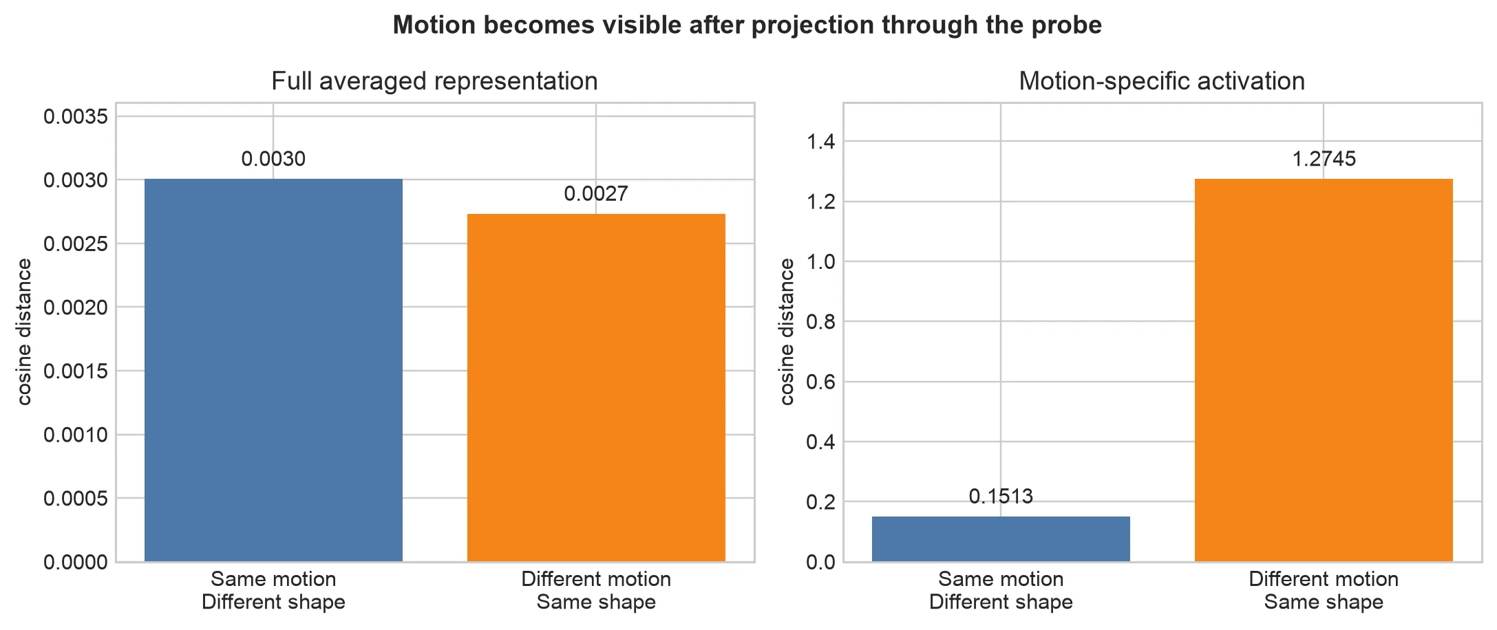
Roughly eight times farther apart once you’re looking in the right place. Same story as an AUC, meaning how often a different-motion pair lands farther apart than a same-motion pair:
| Representation | Motion-separation AUC |
|---|---|
| Full averaged representation | 0.396 |
| Motion-specific activation | 0.993 |
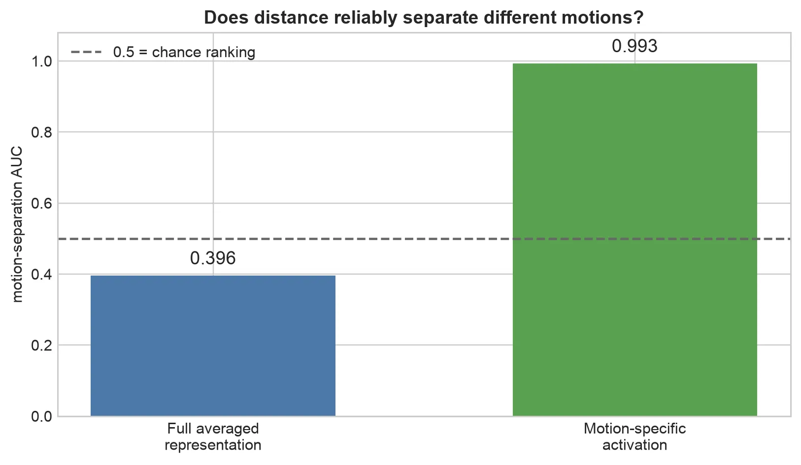
The first comparison asked whether two videos looked similar overall. The probe asked whether their motion looked similar. Those are not the same question. Motion was somewhere in V-JEPA’s frozen representation; averaging everything together just made it hard to see.
Conclusion
So, does V-JEPA understand motion? I don’t think this experiment is enough to say that. These were four shapes moving in four directions with simple backgrounds.
What I can say is that shape and direction are both in there. A linear probe could pull them out without changing V-JEPA, and it could still identify direction when I changed the rendering style or withheld a shape from training.
That was what I wanted from this experiment. Looking at one distance between two whole-video embeddings told me almost nothing. Making the videos stupidly simple and asking a specific question gave me a peek into the representation that kind of worked! Yay.